Management Memory Sistem Operation

 

Memory Management

The main purpose of a computer system is to execute programs. These
programs, together with the data they access, must be at least partially
in main memory during execution.
To improve both the utilization of the CPU and the speed of its
response to users, a general-purpose computer must keep several processes
in memory. Many memory-management schemes exist, reflecting
various approaches, and the effectiveness of each algorithm depends
on the situation. Selection of a memory-management scheme for a system
depends onmany factors, especially on the hardware design of the
system. Most algorithms require hardware support.Main Memory
In Chapter 6, we showed how the CPU can be shared by a set of processes. As
a result of CPU scheduling, we can improve both the utilization of the CPU and
the speed of the computer’s response to its users. To realize this increase in
performance, however, we must keep several processes in memory—that is,
we must share memory.
In this chapter, we discuss various ways to manage memory. The memorymanagement
algorithms vary from a primitive bare-machine approach to
paging and segmentation strategies. Each approach has its own advantages
and disadvantages. Selection of a memory-management method for a specific
system depends on many factors, especially on the hardware design of the
system. As we shall see, many algorithms require hardware support, leading
many systems to have closely integrated hardware and operating-system
memory management.
CHAPTER OBJECTIVES
• To provide a detailed description of various ways of organizing memory
hardware.
• To explore various techniques of allocating memory to processes.
• To discuss in detail how paging works in contemporary computer systems.

8.1 Background
As we saw in Chapter 1, memory is central to the operation of a modern
computer system. Memory consists of a large array of bytes, each with its own
address. The CPU fetches instructions from memory according to the value of
the program counter. These instructions may cause additional loading from
and storing to specific memory addresses.
A typical instruction-execution cycle, for example, first fetches an instruction
from memory. The instruction is then decoded and may cause operands
to be fetched from memory. After the instruction has been executed on the
operands, results may be stored back in memory. The memory unit sees onlythe instruction counter, indexing, indirection, literal addresses, and so on) or
what they are for (instructions or data). Accordingly, we can ignore how a
program generates a memory address. We are interested only in the sequence
of memory addresses generated by the running program.
We begin our discussion by covering several issues that are pertinent
to managing memory: basic hardware, the binding of symbolic memory
addresses to actual physical addresses, and the distinction between logical
and physical addresses.We conclude the section with a discussion of dynamic
linking and shared libraries.

8.1.1 Basic Hardware
Main memory and the registers built into the processor itself are the only
general-purpose storage that the CPU can access directly. There are machine
instructions that take memory addresses as arguments, but none that take disk
addresses. Therefore, any instructions in execution, and any data being used
by the instructions, must be in one of these direct-access storage devices. If the
data are not in memory, they must be moved there before the CPU can operate
on them.
Registers that are built into the CPU are generally accessible within one
cycle of the CPU clock. Most CPUs can decode instructions and perform simple
operations on register contents at the rate of one or more operations per
clock tick. The same cannot be said of main memory, which is accessed via
a transaction on the memory bus. Completing a memory access may take
many cycles of the CPU clock. In such cases, the processor normally needs to
stall, since it does not have the data required to complete the instruction that it
is executing. This situation is intolerable because of the frequency of memory
accesses. The remedy is to add fastmemorybetween the CPUand mainmemory,
typically on the CPU chip for fast access. Such a cache was described in Section
1.8.3. To manage a cache built into the CPU, the hardware automatically speeds
up memory access without any operating-system control.
Not only are we concerned with the relative speed of accessing physical
memory, but we also must ensure correct operation. For proper system
operation we must protect the operating system from access by user processes.
On multiuser systems, we must additionally protect user processes from
one another. This protection must be provided by the hardware because the
operating system doesn’t usually intervene between the CPU and its memory
accesses (because of the resulting performance penalty). Hardware implements
this production in several different ways, as we show throughout the chapter.
Here, we outline one possible implementation.
We first need to make sure that each process has a separate memory space.
Separate per-process memory space protects the processes from each other and
is fundamental to having multiple processes loaded in memory for concurrent
execution. To separate memory spaces, we need the ability to determine the
range of legal addresses that the process may access and to ensure that the
process can access only these legal addresses. We can provide this protection
by using two registers, usually a base and a limit, as illustrated in Figure 8.1.
The base register holds the smallest legal physical memory address; the limit
register specifies the size of the range. For example, if the base register holds







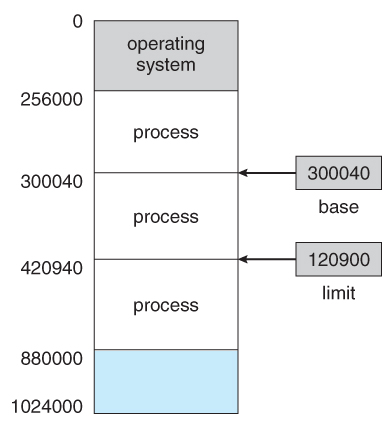
300040 and the limit register is 120900, then the program can legally access all
addresses from 300040 through 420939 (inclusive).
Protection of memory space is accomplished by having the CPU hardware
compare every address generated in user mode with the registers. Any attempt
by a program executing in user mode to access operating-system memory or
other users’ memory results in a trap to the operating system, which treats the
attempt as a fatal error (Figure 8.2). This scheme prevents a user program from
(accidentally or deliberately) modifying the code or data structures of either
the operating system or other users.
The base and limit registers can be loaded only by the operating system,
which uses a special privileged instruction. Since privileged instructions can
be executed only in kernel mode, and since only the operating system executes
in kernel mode, only the operating system can load the base and limit registers.
This scheme allows the operating system to change the value of the registers
but prevents user programs from changing the registers’ contents.
The operating system, executing in kernel mode, is given unrestricted
access to both operating-system memory and users’ memory. This provision
allows the operating system to load users’ programs into users’ memory, to
dump out those programs in case of errors, to access and modify parameters
of system calls, to perform I/O to and from user memory, and to provide
many other services. Consider, for example, that an operating system for a
multiprocessing system must execute context switches, storing the state of one
process from the registers into main memory before loading the next process’s
context from main memory into the registers.

8.1.2 Address Binding
Usually, a program resides on a disk as a binary executable file. To be executed,
the program must be brought into memory and placed within a process.
Depending on the memory management in use, the process may be moved
between disk and memory during its execution. The processes on the disk that
are waiting to be brought into memory for execution form the input queue.
The normal single-tasking procedure is to select one of the processes
in the input queue and to load that process into memory. As the process
is executed, it accesses instructions and data from memory. Eventually, the
process terminates, and its memory space is declared available.
Most systems allow a user process to reside in any part of the physical
memory. Thus, although the address space of the computer may start at 00000,
the first address of the user process need not be 00000. You will see later how
a user program actually places a process in physical memory.
In most cases, a user program goes through several steps—some of which
may be optional—before being executed (Figure 8.3). Addresses may be
represented in different ways during these steps. Addresses in the source
program are generally symbolic (such as the variable count). A compiler
typically binds these symbolic addresses to relocatable addresses (such as
“14 bytes from the beginning of this module”). The linkage editor or loader
in turn binds the relocatable addresses to absolute addresses (such as 74014).
Each binding is a mapping from one address space to another.
Classically, the binding of instructions and data to memory addresses can
be done at any step along the way:
      • Compile time. If you know at compile time where the process will reside
in memory, then absolute code can be generated. For example, if you know
that a user process will reside starting at location R, then the generated
compiler code will start at that location and extend up from there. If, at
some later time, the starting location changes, then it will be necessary
to recompile this code. The MS-DOS .COM-format programs are bound at
compile time.
     • Load time. If it is not known at compile time where the process will reside
in memory, then the compiler must generate relocatable code. In this case,
final binding is delayed until load time. If the starting address changes, we

need only reload the user code to incorporate this changed value.


• Execution time. If the process can be moved during its execution from
one memory segment to another, then binding must be delayed until run
time. Special hardware must be available for this scheme to work, as will
be discussed in Section 8.1.3. Most general-purpose operating systems use
this method.
Amajor portion of this chapter is devoted to showing how these various bindings
can be implemented effectively in a computer system and to discussing
appropriate hardware support.
 
8.1.3 Logical Versus Physical Address Space
An address generated by the CPU is commonly referred to as a logical address,
whereas an address seen by the memory unit—that is, the one loaded into
the memory-address register of the memory—is commonly referred to as a
physical address.
The compile-time and load-time address-binding methods generate identical
logical and physical addresses. However, the execution-time address

binding scheme results in differing logical and physical addresses. In this
case, we usually refer to the logical address as a virtual address. We use
logical address and virtual address interchangeably in this text. The set of all
logical addresses generated by a program is a logical address space. The set
of all physical addresses corresponding to these logical addresses is a physical
address space. Thus, in the execution-time address-binding scheme, the logical
and physical address spaces differ.
The run-time mapping from virtual to physical addresses is done by a
hardware device called the memory-management unit (MMU).We can choose
from many different methods to accomplish such mapping, as we discuss in
Section 8.3 through Section 8.5. For the time being, we illustrate this mapping
with a simple MMU scheme that is a generalization of the base-register scheme
described in Section 8.1.1. The base register is now called a relocation register.
The value in the relocation register is added to every address generated by a
user process at the time the address is sent to memory (see Figure 8.4). For
example, if the base is at 14000, then an attempt by the user to address location
0 is dynamically relocated to location 14000; an access to location 346 is mapped
to location 14346.
The user program never sees the real physical addresses. The program can
create a pointer to location 346, store it in memory, manipulate it, and compare it
with other addresses—all as the number 346. Only when it is used as a memory
address (in an indirect load or store, perhaps) is it relocated relative to the base
register. The user program deals with logical addresses. The memory-mapping
hardware converts logical addresses into physical addresses. This form of
execution-time binding was discussed in Section 8.1.2. The final location of
a referenced memory address is not determined until the reference is made.
We now have two different types of addresses: logical addresses (in the
range 0 to max) and physical addresses (in the range R + 0 to R + max for a base
value R). The user program generates only logical addresses and thinks that
the process runs in locations 0 to max. However, these logical addresses must
be mapped to physical addresses before they are used. The concept of a logicaladdress space that is bound to a separate physical address space is central to
proper memory management.
 
8.1.4 Dynamic Loading
In our discussion so far, it has been necessary for the entire program and all
data of a process to be in physical memory for the process to execute. The size
of a process has thus been limited to the size of physical memory. To obtain
better memory-space utilization, we can use dynamic loading. With dynamic
loading, a routine is not loaded until it is called. All routines are kept on disk
in a relocatable load format. The main program is loaded into memory and
is executed. When a routine needs to call another routine, the calling routine
first checks to see whether the other routine has been loaded. If it has not, the
relocatable linking loader is called to load the desired routine into memory and
to update the program’s address tables to reflect this change. Then control is
passed to the newly loaded routine.
The advantage of dynamic loading is that a routine is loaded only when it
is needed. This method is particularly useful when large amounts of code are
needed to handle infrequently occurring cases, such as error routines. In this
case, although the total program size may be large, the portion that is used
(and hence loaded) may be much smaller.
Dynamic loading does not require special support from the operating
system. It is the responsibility of the users to design their programs to take
advantage of such a method. Operating systems may help the programmer,
however, by providing library routines to implement dynamic loading.
 
8.1.5 Dynamic Linking and Shared Libraries
Dynamically linked libraries are system libraries that are linked to user
programs when the programs are run (refer back to Figure 8.3). Some operating
systems support only static linking, in which system libraries are treated
like any other object module and are combined by the loader into the binary
program image. Dynamic linking, in contrast, is similar to dynamic loading.
Here, though, linking, rather than loading, is postponed until execution time.
This feature is usually used with system libraries, such as language subroutine
libraries. Without this facility, each program on a system must include a copy
of its language library (or at least the routines referenced by the program) in the
executable image. This requirementwastes both disk space and main memory.
With dynamic linking, a stub is included in the image for each libraryroutine
reference. The stub is a small piece of code that indicates how to locate
the appropriate memory-resident library routine or how to load the library if
the routine is not already present. When the stub is executed, it checks to see
whether the needed routine is already in memory. If it is not, the program loads
the routine into memory. Either way, the stub replaces itself with the address
of the routine and executes the routine. Thus, the next time that particular
code segment is reached, the library routine is executed directly, incurring no
cost for dynamic linking. Under this scheme, all processes that use a language
library execute only one copy of the library code.
This feature can be extended to library updates (such as bug fixes).Alibrary
may be replaced by a new version, and all programs that reference the libraryprograms would need to be relinked to gain access to the new library. So that
programs will not accidentally execute new, incompatible versions of libraries,
version information is included in both the program and the library.More than
one version of a library may be loaded into memory, and each program uses its
version information to decide which copy of the library to use. Versions with
minor changes retain the same version number, whereas versions with major
changes increment the number. Thus, only programs that are compiled with
the new library version are affected by any incompatible changes incorporated
in it. Other programs linked before the new library was installed will continue
using the older library. This system is also known as shared libraries.
Unlike dynamic loading, dynamic linking and shared libraries generally
require help from the operating system. If the processes in memory are
protected fromone another, then the operating system is the only entity that can
check to see whether the needed routine is in another process’s memory space
or that can allow multiple processes to access the same memory addresses.We
elaborate on this concept when we discuss paging in Section 8.5.4.
will automatically use the new version. Without dynamic linking, all such

8.2 Swapping
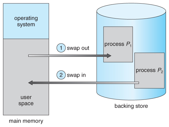
     A process must be in memory to be executed. A process, however, can be
swapped temporarily out of memory to a backing store and then brought back
into memory for continued execution (Figure 8.5). Swapping makes it possible
for the total physical address space of all processes to exceed the real physical
memory of the system, thus increasing the degree of multiprogramming in a
system.
 
8.2.1 Standard Swapping
Standard swapping involves moving processes between main memory and
a backing store. The backing store is commonly a fast disk. It must be large
enough to accommodate copies of all memory images for all users, and it must
provide direct access to these memory images. The system maintains a ready
queue consisting of all processes whose memory images are on the backing
store or in memory and are ready to run. Whenever the CPU scheduler decides
to execute a process, it calls the dispatcher. The dispatcher checks to see whether
the next process in the queue is in memory. If it is not, and if there is no free
memory region, the dispatcher swaps out a process currently in memory and
swaps in the desired process. It then reloads registers and transfers control to
the selected process.
The context-switch time in such a swapping system is fairly high. To get an
idea of the context-switch time, let’s assume that the user process is 100 MB in
size and the backing store is a standard hard disk with a transfer rate of 50 MB
per second. The actual transfer of the 100-MB process to or from main memory
takes
100 MB/50 MB per second = 2 seconds
The swap time is 200 milliseconds. Since we must swap both out and in, the
total swap time is about 4,000 milliseconds. (Here, we are ignoring other disk
performance aspects, which we cover in Chapter 10.)
Notice that the major part of the swap time is transfer time. The total
transfer time is directly proportional to the amount of memory swapped.
If we have a computer system with 4 GB of main memory and a resident
operating system taking 1 GB, the maximum size of the user process is 3
GB. However, many user processes may be much smaller than this—say, 100
MB. A 100-MB process could be swapped out in 2 seconds, compared with
the 60 seconds required for swapping 3 GB. Clearly, it would be useful to
know exactly how much memory a user process is using, not simply how
much it might be using. Then we would need to swap only what is actually
used, reducing swap time. For this method to be effective, the user must
keep the system informed of any changes in memory requirements. Thus,
a process with dynamic memory requirements will need to issue system calls
(request memory() and release memory()) to inform the operating system
of its changing memory needs.
Swapping is constrained by other factors as well. If we want to swap
a process, we must be sure that it is completely idle. Of particular concern
is any pending I/O. A process may be waiting for an I/O operation when
we want to swap that process to free up memory. However, if the I/O is
asynchronously accessing the user memory for I/O buffers, then the process
cannot be swapped. Assume that the I/O operation is queued because the
device is busy. If we were to swap out process P1 and swap in process P2, the
I/O operation might then attempt to use memory that now belongs to process
P2. There are two main solutions to this problem: never swap a process with
pending I/O, or execute I/O operations only into operating-system buffers.
Transfers between operating-system buffers and process memory then occur
only when the process is swapped in. Note that this double buffering itself
adds overhead. We now need to copy the data again, from kernel memory to
user memory, before the user process can access it.
Standard swapping is not used in modern operating systems. It requires too
much swapping time and provides too little execution time to be a reasonablememory-management solution. Modified versions of swapping, however, are
found on many systems, including UNIX, Linux, andWindows. In one common
variation, swapping is normally disabled but will start if the amount of free
memory (unused memory available for the operating system or processes to
use) falls below a threshold amount. Swapping is halted when the amount
of free memory increases. Another variation involves swapping portions of
processes—rather than entire processes—to decrease swap time. Typically,
these modified forms of swapping work in conjunction with virtual memory,
which we cover in Chapter 9.
 
8.2.2 Swapping on Mobile Systems
Although most operating systems for PCs and servers support some modified
version of swapping, mobile systems typically do not support swapping in any
form. Mobile devices generally use flash memory rather than more spacious
hard disks as their persistent storage. The resulting space constraint is one
reason why mobile operating-system designers avoid swapping. Other reasons
include the limited number of writes that flash memory can tolerate before it
becomes unreliable and the poor throughput between main memory and flash
memory in these devices.
Instead of using swapping, when free memory falls below a certain
threshold, Apple’s iOS asks applications to voluntarily relinquish allocated
memory. Read-only data (such as code) are removed from the system and later
reloaded from flash memory if necessary. Data that have been modified (such
as the stack) are never removed. However, any applications that fail to free up
sufficient memory may be terminated by the operating system.
Android does not support swapping and adopts a strategy similar to that
used by iOS. It may terminate a process if insufficient free memory is available.
However, before terminating a process, Android writes its application state to
flash memory so that it can be quickly restarted.
Because of these restrictions, developers for mobile systems must carefully
allocate and release memory to ensure that their applications do not use too
much memory or suffer from memory leaks. Note that both iOS and Android
support paging, so they do have memory-management abilities. We discuss
paging later in this chapter.
 
8.3 Contiguous Memory Allocation
The main memory must accommodate both the operating system and the
various user processes.We therefore need to allocate main memory in themost
efficient way possible. This section explains one early method, contiguous
memory allocation.
The memory is usually divided into two partitions: one for the resident
operating system and one for the user processes. We can place the operating
system in either low memory or high memory. The major factor affecting this
decision is the location of the interrupt vector. Since the interrupt vector is
often in low memory, programmers usually place the operating system in low
memory as well. Thus, in this text, we discuss only the situation in whichthe operating system resides in low memory. The development of the other
situation is similar.
We usually want several user processes to reside in memory at the same
time. We therefore need to consider how to allocate available memory to the
processes that are in the input queue waiting to be brought into memory. In
contiguous memory allocation, each process is contained in a single section of
memory that is contiguous to the section containing the next process.
 
8.3.1 Memory Protection
Before discussing memory allocation further, we must discuss the issue of
memory protection. We can prevent a process from accessing memory it does
not own by combining two ideas previously discussed. If we have a system
with a relocation register (Section 8.1.3), together with a limit register (Section
8.1.1), we accomplish our goal. The relocation register contains the value of
the smallest physical address; the limit register contains the range of logical
addresses (for example, relocation = 100040 and limit = 74600). Each logical
address must fall within the range specified by the limit register. The MMU
maps the logical address dynamically by adding the value in the relocation
register. This mapped address is sent to memory (Figure 8.6).
When the CPU scheduler selects a process for execution, the dispatcher
loads the relocation and limit registers with the correct values as part of the
context switch. Because every address generated by a CPU is checked against
these registers, we can protect both the operating system and the other users’
programs and data from being modified by this running process.
The relocation-register scheme provides an effective way to allow the
operating system’s size to change dynamically. This flexibility is desirable in
many situations. For example, the operating system contains code and buffer
space for device drivers. If a device driver (or other operating-system service)
is not commonly used, we do not want to keep the code and data inmemory, as
we might be able to use that space for other purposes. Such code is sometimes
called transient operating-system code; it comes and goes as needed. Thus,
using this code changes the size of the operating system during program


8.3.2 Memory Allocation
Now we are ready to turn to memory allocation. One of the simplest
methods for allocating memory is to divide memory into several fixed-sized
partitions. Each partition may contain exactly one process. Thus, the degree
of multiprogramming is bound by the number of partitions. In this multiplepartition
method, when a partition is free, a process is selected from the input
queue and is loaded into the free partition. When the process terminates, the
partition becomes available for another process. This method was originally
used by the IBM OS/360 operating system (called MFT)but is no longer in use.
The method described next is a generalization of the fixed-partition scheme
(called MVT); it is used primarily in batch environments. Many of the ideas
presented here are also applicable to a time-sharing environment in which
pure segmentation is used for memory management (Section 8.4).
In the variable-partition scheme, the operating system keeps a table
indicating which parts of memory are available and which are occupied.
Initially, all memory is available for user processes and is considered one
large block of available memory, a hole. Eventually, as you will see, memory
contains a set of holes of various sizes.
As processes enter the system, they are put into an input queue. The
operating system takes into account the memory requirements of each process
and the amount of available memory space in determining which processes are
allocated memory. When a process is allocated space, it is loaded into memory,
and it can then compete for CPU time. When a process terminates, it releases its
memory, which the operating system may then fill with another process from
the input queue.
At any given time, then, we have a list of available block sizes and an
input queue. The operating system can order the input queue according to
a scheduling algorithm. Memory is allocated to processes until, finally, the
memory requirements of the next process cannot be satisfied—that is, no
available block of memory (or hole) is large enough to hold that process. The
operating system can then wait until a large enough block is available, or it can
skip down the input queue to see whether the smaller memory requirements
of some other process can be met.
In general, as mentioned, the memory blocks available comprise a set of
holes of various sizes scattered throughout memory. When a process arrives
and needs memory, the system searches the set for a hole that is large enough
for this process. If the hole is too large, it is split into two parts. One part is
allocated to the arriving process; the other is returned to the set of holes. When
a process terminates, it releases its block of memory, which is then placed back
in the set of holes. If the new hole is adjacent to other holes, these adjacent holes
are merged to form one larger hole. At this point, the system may need to check
whether there are processes waiting for memory and whether this newly freed
and recombined memory could satisfy the demands of any of these waiting
processes.
This procedure is a particular instance of the general dynamic storageallocation
problem, which concerns how to satisfy a request of size n from a
list of free holes. There are many solutions to this problem. The first-fit, best-fit,
and worst-fit strategies are the ones most commonly used to select a free hole• First fit. Allocate the first hole that is big enough. Searching can start either
at the beginning of the set of holes or at the location where the previous
first-fit search ended.We can stop searching as soon as we find a free hole
that is large enough.
• Best fit. Allocate the smallest hole that is big enough. We must search the
entire list, unless the list is ordered by size. This strategy produces the
smallest leftover hole.
• Worst fit. Allocate the largest hole. Again, we must search the entire list,
unless it is sorted by size. This strategy produces the largest leftover hole,
which may be more useful than the smaller leftover hole from a best-fit
approach.
Simulations have shown that both first fit and best fit are better than worst
fit in terms of decreasing time and storage utilization. Neither first fit nor best
fit is clearly better than the other in terms of storage utilization, but first fit is
generally faster.
 
8.3.3 Fragmentation
Both the first-fit and best-fit strategies for memory allocation suffer from
external fragmentation. As processes are loaded and removed from memory,
the free memory space is broken into little pieces. External fragmentation exists
when there is enough total memory space to satisfy a request but the available
spaces are not contiguous: storage is fragmented into a large number of small
holes. This fragmentation problem can be severe. In the worst case, we could
have a block of free (or wasted) memory between every two processes. If all
these small pieces of memory were in one big free block instead, we might be
able to run several more processes.
Whether we are using the first-fit or best-fit strategy can affect the amount
of fragmentation. (First fit is better for some systems, whereas best fit is better
for others.) Another factor is which end of a free block is allocated. (Which is
the leftover piece—the one on the top or the one on the bottom?) No matter
which algorithm is used, however, external fragmentation will be a problem.
Depending on the total amount of memory storage and the average process
size, external fragmentation may be a minor or a major problem. Statistical
analysis of first fit, for instance, reveals that, even with some optimization,
given N allocated blocks, another 0.5 N blocks will be lost to fragmentation.
That is, one-third of memory may be unusable! This property is known as the
50-percent rule.
Memory fragmentation can be internal as well as external. Consider a
multiple-partition allocation scheme with a hole of 18,464 bytes. Suppose that
the next process requests 18,462 bytes. Ifweallocate exactly the requested block,
we are left with a hole of 2 bytes. The overhead to keep track of this hole will be
substantially larger than the hole itself. The general approach to avoiding this
problem is to break the physical memory into fixed-sized blocks and allocate
memory in units based on block size.With this approach, the memory allocated
to a process may be slightly larger than the requested memory. The difference
between these two numbers is internal fragmentation—unused memory that
is internal to a partition.• First fit. Allocate the first hole that is big enough. Searching can start either
at the beginning of the set of holes or at the location where the previous
first-fit search ended.We can stop searching as soon as we find a free hole
that is large enough.
• Best fit. Allocate the smallest hole that is big enough. We must search the
entire list, unless the list is ordered by size. This strategy produces the
smallest leftover hole.
• Worst fit. Allocate the largest hole. Again, we must search the entire list,
unless it is sorted by size. This strategy produces the largest leftover hole,
which may be more useful than the smaller leftover hole from a best-fit
approach.
Simulations have shown that both first fit and best fit are better than worst
fit in terms of decreasing time and storage utilization. Neither first fit nor best
fit is clearly better than the other in terms of storage utilization, but first fit is
generally faster.
8.3.3 Fragmentation
Both the first-fit and best-fit strategies for memory allocation suffer from
external fragmentation. As processes are loaded and removed from memory,
the free memory space is broken into little pieces. External fragmentation exists
when there is enough total memory space to satisfy a request but the available
spaces are not contiguous: storage is fragmented into a large number of small
holes. This fragmentation problem can be severe. In the worst case, we could
have a block of free (or wasted) memory between every two processes. If all
these small pieces of memory were in one big free block instead, we might be
able to run several more processes.
Whether we are using the first-fit or best-fit strategy can affect the amount
of fragmentation. (First fit is better for some systems, whereas best fit is better
for others.) Another factor is which end of a free block is allocated. (Which is
the leftover piece—the one on the top or the one on the bottom?) No matter
which algorithm is used, however, external fragmentation will be a problem.
Depending on the total amount of memory storage and the average process
size, external fragmentation may be a minor or a major problem. Statistical
analysis of first fit, for instance, reveals that, even with some optimization,
given N allocated blocks, another 0.5 N blocks will be lost to fragmentation.
That is, one-third of memory may be unusable! This property is known as the
50-percent rule.
Memory fragmentation can be internal as well as external. Consider a
multiple-partition allocation scheme with a hole of 18,464 bytes. Suppose that
the next process requests 18,462 bytes. Ifweallocate exactly the requested block,
we are left with a hole of 2 bytes. The overhead to keep track of this hole will be
substantially larger than the hole itself. The general approach to avoiding this
problem is to break the physical memory into fixed-sized blocks and allocate
memory in units based on block size.With this approach, the memory allocated
to a process may be slightly larger than the requested memory. The difference
between these two numbers is internal fragmentation—unused memory that
is internal to a partition.One solution to the problem of external fragmentation is compaction. The
goal is to shuffle the memory contents so as to place all free memory together
in one large block. Compaction is not always possible, however. If relocation
is static and is done at assembly or load time, compaction cannot be done. It is
possible only if relocation is dynamic and is done at execution time. If addresses
are relocated dynamically, relocation requires only moving the program and
data and then changing the base register to reflect the new base address. When
compaction is possible, we must determine its cost. The simplest compaction
algorithm is to move all processes toward one end of memory; all holes move in
the other direction, producing one large hole of available memory. This scheme
can be expensive.
Another possible solution to the external-fragmentation problem is to
permit the logical address space of the processes to be noncontiguous, thus
allowing a process to be allocated physical memory wherever such memory is
available. Two complementary techniques achieve this solution: segmentation
(Section 8.4) and paging (Section 8.5). These techniques can also be combined.
Fragmentation is a general problem in computing that can occur wherever
we must manage blocks of data. We discuss the topic further in the storage
management chapters (Chapters 10 through and 12).